Summarize only filtered values using SUBTOTAL & AGGREGATE formulas

We all know the good old SUM() formula. It can sum up values in a range. But what if you want to sum up only filtered values in a range? SUM() doesn’t care if a value is filtered or not. It just sums up the numbers. But there are other formulas that can pay attention to the filters. Let’s learn about them.

What is VLOOKUP Formula & How to use it?

Learning VLOOKUP formulas will change your basic approach towards data. You will suddenly feel that you have discovered a superman cape in your attic. It is that real awesome.

What does VLOOKUP really do?

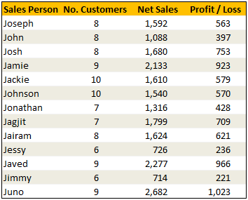
Imagine you have a list of data like this:

Now, how do you answer the question – “How many sales did Jimmy make?“

Yes, your guess is right. VLOOKUP is one of the formulas you can use to answer questions like this.

VLOOKUP searches a list for a value in left most column and returns corresponding value from adjacent columns.

So, in our case, we need VLOOKUP to search for Jimmy and return the amount of sales he made from column 3.

VLOOKUP Syntax:

The syntax of VLOOKUP is simple:

=VLOOKUP( this value, your data table, column number, optional is your table sorted?)

How Will You Benefit From Learning Exel?

Excel Shortcuts for PC & Mac

Excel - Pivot Tables & Charts

Multiply using PasteSpecial

This post will help you learn a smarter way to multiply a range of data with a single number. For example below in Column A we have 5 products and column B contains their corresponding price.

Now if you want to multiply the price by say 10%. You can do that smartly,  using the method I am going tell.  Enter 1.1 into any blank cell (like D1)

Select the cell and choose Edit, Copy. Select the range of values and choose Edit, Paste Special.

Choose the Multiply option and click OK.

Delete the cell that contains the 1.1.  Your final result will look like this.